This page was generated from docs/source/examples/example_3D_DYCOMS.ipynb.
3D Structure Function Data with DYCOMS LES
This example will guide you through each step necessary to compute Longitudinal SFs from DYCOMS Data
\(\textbf{General procedure}:\)
1 -  Load 3D DYCOMS dataset, dataset can be made available upon reasonable request
2 -  Format dataset
3 -  Compute 3D longitudinal SF
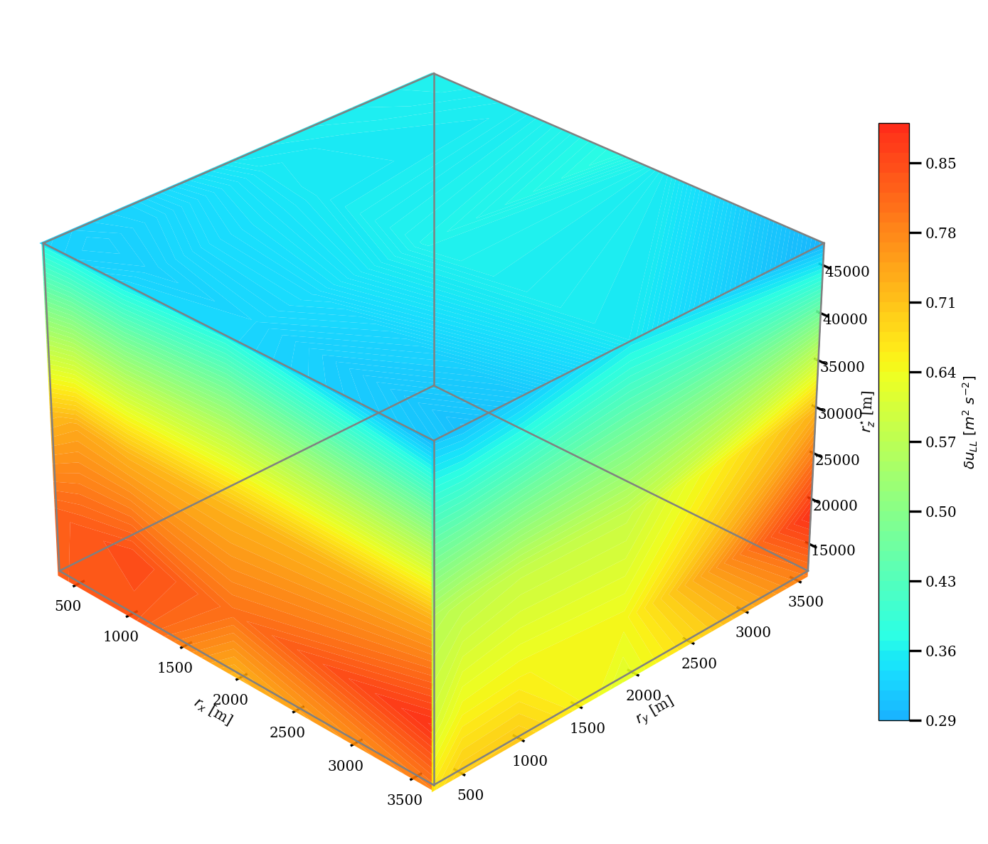
4 -  Plot 3D longitudinal SF
5 -  Compute Isotropic SF
6 -  Plot Isotropic SF
\(\textbf{Note}:\) To capture meaningful Structure functions in 3D, the vertical coordinate should be stretched as
\(z^{*} = \int_{0}^{z} \frac{\overline{N}}{f} dz^{'}\) where N is derived from the 3D Brunt-Vaisala frequency and f is the Coriolis parameter
\(\textbf{Motivation}:\)
This example extends the 2D structure function analysis to fully three-dimensional DYCOMS stratocumulus data, providing a complete characterization of turbulence anisotropy in the cloud-topped boundary layer. While 2D analysis captures horizontal turbulent structures, the 3D approach reveals the critical vertical variations in turbulence characteristics from the well-mixed convective region to the stably stratified inversion layer.
\(\textbf{Reference}:\)
Matheou, G., & Chung, D. (2014). Large-eddy simulation of stratified turbulence. Part II: Application of the stretched-vortex model to the atmospheric boundary layer. Journal of the Atmospheric Sciences, 71(12), 4439-4460. https://doi.org/10.1175/JAS-D-13-0306.1
[158]:
import xarray as xr
import matplotlib.pyplot as plt
from matplotlib.colors import LogNorm, SymLogNorm, Normalize
import matplotlib.ticker as ticker
import pyturbo_sf as psf
import numpy as np
import dask.array as da
import matplotlib.pyplot as plt

linewidth = 2
fontsize = 12
plt.rcParams['xtick.labelsize'] = fontsize
plt.rcParams['ytick.labelsize'] = fontsize
plt.rcParams['xtick.major.width'] = 2
plt.rcParams['xtick.minor.width'] = 2
plt.rcParams['ytick.major.width'] = 2
plt.rcParams['ytick.minor.width'] = 2
plt.rcParams['xtick.major.size'] = 10
plt.rcParams['xtick.minor.size'] = 5
plt.rcParams['ytick.major.size'] = 10
plt.rcParams['ytick.minor.size'] = 5
plt.rcParams['savefig.dpi'] = 150
plt.rc('font', family='serif')
import gc
Load Dataset
[2]:
path = '/glade/derecho/scratch/aayouche/LES/outputs/'
ds_u = xr.open_zarr(path+'u_dycoms.zarr')
ds_v = xr.open_zarr(path+'v_dycoms.zarr')
ds_w = xr.open_zarr(path+'w_dycoms.zarr')
ds_b = xr.open_zarr(path+'buoyancy_dycoms.zarr')
xt = ds_u.x + ds_u.x.max()
yt = ds_u.y + ds_u.y.max()
zt = ds_v.z
N = (xr.apply_ufunc(np.abs,ds_b.buoyancy.differentiate('z').transpose('z','y','x'),dask='parallelized')**0.5).mean(('y','x'))
f = 1.0e-4
u = ds_u['u'].transpose('z','y','x')
v = ds_v['v'].transpose('z','y','x')
w = ds_w['w'].transpose('z','y','x')
y_coord = yt.expand_dims({'z': len(zt), 'x': len(xt)}).transpose('z','y','x').drop_vars('y')
x_coord = xt.expand_dims({'z': len(zt), 'y': len(yt)}).transpose('z','y','x').drop_vars('x')
Compute \(Z^{\star}\)
[3]:
def calculate_stretched_coordinate_1D(z_coord, N_field, f_scalar, surface_at_top=True):
    """
    Calculate the stretched coordinate Z* = ∫(N/f)dz' between free surface (eta) and z
    Optimized for case where:
    - z_coord is 1D (varies only with depth)
    - N_field is 1D (varies only with depth)
    - f_scalar is a constant scalar value

    Parameters:
    -----------
    z_coord : xarray.DataArray
        The 1D z-coordinate array with dimension 'z'
    N_field : xarray.DataArray
        The 1D Brunt-Väisälä frequency array with dimension 'z'
    f_scalar : float or xarray.DataArray with single value
        The Coriolis parameter as a scalar
    surface_at_top : bool, optional
        If True, assumes the free surface (eta) is at z_coord[0]
        If False, assumes the free surface is at z_coord[-1]

    Returns:
    --------
    Z_star : xarray.DataArray
        The 1D stretched coordinate array with dimension 'z'
    """
    # Convert everything to numpy arrays for calculation
    z_values = z_coord.values
    N_values = N_field.values
    f_value = float(f_scalar)  # Ensure it's a scalar

    # Calculate N/f directly - no need for loops
    N_over_f = N_values / f_value

    # Create output array
    Z_star_values = np.zeros_like(z_values)

    # Determine surface index
    surface_idx = 0 if surface_at_top else len(z_values) - 1

    # For each depth level, integrate from surface to that depth
    for k in range(len(z_values)):
        if k == surface_idx:
            Z_star_values[k] = 0.0
        else:
            if surface_at_top:
                # Integrate downward from surface
                if k > surface_idx:
                    z_section = z_values[surface_idx:k+1]
                    Nf_section = N_over_f[surface_idx:k+1]
                    Z_star_values[k] = np.trapz(Nf_section, z_section)
                else:
                    z_section = z_values[k:surface_idx+1]
                    Nf_section = N_over_f[k:surface_idx+1]
                    Z_star_values[k] = -np.trapz(Nf_section, z_section)
            else:
                # Integrate upward from depth to surface
                if k < surface_idx:
                    z_section = z_values[k:surface_idx+1]
                    Nf_section = N_over_f[k:surface_idx+1]
                    Z_star_values[k] = np.trapz(Nf_section, z_section)
                else:
                    z_section = z_values[surface_idx:k+1]
                    Nf_section = N_over_f[surface_idx:k+1]
                    Z_star_values[k] = -np.trapz(Nf_section, z_section)

    # Create xarray DataArray with the same dimension and coordinates as z_coord
    Z_star = xr.DataArray(
        Z_star_values,
        dims=z_coord.dims,
        coords=z_coord.coords,
        attrs={'long_name': 'Stretched coordinate Z*',
               'units': 'm',
               'description': 'Stretched coordinate Z* = ∫(N/f)dz\''}
    )

    return Z_star

# First compute the 1D stretched coordinate
Z_star_1D = calculate_stretched_coordinate_1D(
    z_coord=zt,  # Your 1D z-coordinate
    N_field=N,        # Your 1D N profile
    f_scalar=f,       # Your scalar f value
    surface_at_top=True
)

z_coord = Z_star_1D.expand_dims({'y': len(yt), 'x': len(xt)}).transpose('z','y','x').drop_vars('z')
Format Dataset
[4]:
ds = xr.Dataset(
    data_vars={
        'u': u,  # These are DataArrays - correct usage
        'v': v,
        'w': w
    },
    coords={
        'z': z_coord,  # These are your coordinate DataArrays
        'y': y_coord,
        'x': x_coord
    }
)
[160]:
ds
[160]:
<xarray.Dataset> Size: 966GB
Dimensions:  (z: 1200, y: 4096, x: 4096)
Coordinates:
    x        (z, y, x) float64 161GB 0.0 1.25 2.5 ... 5.118e+03 5.119e+03
    y        (z, y, x) float64 161GB 0.0 0.0 0.0 ... 5.119e+03 5.119e+03
    z        (z, y, x) float64 161GB 0.0 0.0 0.0 ... 6.817e+04 6.817e+04
Data variables:
    u        (z, y, x) float64 161GB dask.array<chunksize=(75, 128, 128), meta=np.ndarray>
    v        (z, y, x) float64 161GB dask.array<chunksize=(75, 128, 128), meta=np.ndarray>
w (z, y, x) float64 161GB dask.array<chunksize=(75, 128, 128), meta=np.ndarray>Calculate 3D Longitudinal SF
[13]:
bins = {
    'x': np.logspace(np.log10(1.25), np.log10(5.0e3), 14),
    'y': np.logspace(np.log10(1.25), np.log10(5.0e3), 14),
    'z': np.logspace(np.log10(320.), np.log10(60.0e3), 12),
}
sf_result = psf.bin_sf_3d(
    ds=ds,
    variables_names=["u","v","w"],
    order=2,
    bins=bins,
    fun='longitudinal',
    bootsize={'z':4,'y':16,'x':16},
    initial_nbootstrap=100,
    max_nbootstrap=200,
    step_nbootstrap=50,
    convergence_eps=1.0,
    n_jobs=128, # number of physical cores / change it to -1 if you want to use logical cores
)
Dimensions ['z', 'y', 'x'] are already in the expected order
Using bootsize: {'z': 4, 'y': 16, 'x': 16}
Bootstrappable dimensions: ['z', 'y', 'x']
All three dimensions ['z', 'y', 'x'] are bootstrappable. Available spacings: [1, 2, 4, 8, 16, 32, 64, 128, 256]

============================================================
STARTING BIN_SF_3D WITH FUNCTION TYPE: longitudinal
Variables: ['u', 'v', 'w'], Order: 2
Bootstrap parameters: initial=100, max=200, step=50
Convergence threshold: 1.0
Bootstrappable dimensions: ['z', 'y', 'x'] (count: 3)
============================================================

Bin dimensions: z=11, y=13, x=13
Total bins: 1859
Bin type for x: logarithmic
Bin type for y: logarithmic
Bin type for z: logarithmic
Available spacings: [1, 2, 4, 8, 16, 32, 64, 128, 256]

INITIAL BOOTSTRAP PHASE
  Processing spacing 1 with 11 bootstraps
  Processing spacing 2 with 11 bootstraps
  Processing spacing 4 with 11 bootstraps
  Processing spacing 8 with 11 bootstraps
  Processing spacing 16 with 11 bootstraps
  Processing spacing 32 with 11 bootstraps
  Processing spacing 64 with 11 bootstraps
  Processing spacing 128 with 11 bootstraps
  Processing spacing 256 with 11 bootstraps

CALCULATING BIN DENSITIES
Total points collected: 101376
Bins with points: 770/1859
Maximum density bin has 2335 points

CALCULATING INITIAL STATISTICS
Marked 1208 low-density bins (< 10 points) as converged
Marked 182 bins with NaN standard deviations as converged
Marked 0 bins with NaN standard deviations as converged
Marked 463 bins as early-converged (std <= 1.0)

STARTING ADAPTIVE CONVERGENCE LOOP

Iteration 1 - 6 unconverged bins

Processing bin (0,7,7) - Density: 0.0004 - Current bootstraps: 100 - Current std: 1.062820 - Points: 971
  Adding 50 more bootstraps to bin (0,7,7)
  Processing spacing 8 with 25 bootstraps
  Processing spacing 16 with 18 bootstraps
  Processing spacing 32 with 5 bootstraps

Processing bin (1,7,7) - Density: 0.0001 - Current bootstraps: 100 - Current std: 0.956592 - Points: 300
  Adding 50 more bootstraps to bin (1,7,7)
  Processing spacing 8 with 41 bootstraps
  Processing spacing 16 with 8 bootstraps
  Bin (1,7,7) CONVERGED after additional bootstraps with std 0.961403 <= 1.0

Processing bin (0,8,8) - Density: 0.0001 - Current bootstraps: 100 - Current std: 1.059169 - Points: 592
  Adding 50 more bootstraps to bin (0,8,8)
  Processing spacing 16 with 29 bootstraps
  Processing spacing 32 with 14 bootstraps
  Processing spacing 64 with 3 bootstraps
  Bin (0,8,8) CONVERGED after additional bootstraps with std 0.915433 <= 1.0

Processing bin (2,7,3) - Density: 0.0000 - Current bootstraps: 100 - Current std: 0.575526 - Points: 25
  Adding 50 more bootstraps to bin (2,7,3)
  Processing spacing 8 with 50 bootstraps
  Bin (2,7,3) CONVERGED after additional bootstraps with std 0.476689 <= 1.0

Processing bin (2,9,9) - Density: 0.0000 - Current bootstraps: 100 - Current std: 0.786950 - Points: 180
  Adding 50 more bootstraps to bin (2,9,9)
  Processing spacing 32 with 50 bootstraps
  Bin (2,9,9) CONVERGED after additional bootstraps with std 0.675540 <= 1.0

Processing bin (4,9,9) - Density: 0.0000 - Current bootstraps: 100 - Current std: 0.827095 - Points: 352
  Adding 50 more bootstraps to bin (4,9,9)
  Processing spacing 32 with 35 bootstraps
  Processing spacing 64 with 14 bootstraps
  Bin (4,9,9) CONVERGED after additional bootstraps with std 0.883059 <= 1.0

Iteration 2 - 1 unconverged bins

Processing bin (0,7,7) - Density: 0.0004 - Current bootstraps: 148 - Current std: 0.952465 - Points: 971
  Adding 50 more bootstraps to bin (0,7,7)
  Processing spacing 8 with 25 bootstraps
  Processing spacing 16 with 18 bootstraps
  Processing spacing 32 with 5 bootstraps
  Bin (0,7,7) CONVERGED after additional bootstraps with std 0.966402 <= 1.0
All bins have converged or reached max bootstraps!

FINAL CONVERGENCE STATISTICS:
  Total bins with data more than 10 points: 651
  Converged bins: 651
  Unconverged bins: 0
  Bins at max bootstraps: 0

Creating output dataset...
3D SF COMPLETED SUCCESSFULLY!
============================================================
Plot 3D Longitudinal SF
[159]:
def plot_sf_3d_box_custom(
        sf_result,
        cmap='jet',
        vmin=0.0,
        vmax=1.0,
        figsize=(12, 10),
        log_color=False,
        log_axes=False,
        z_offset=10e3,
        y_offset=300,
        x_min=300,
        y_min=300,
        elev=30,
        azim=-45,
        corner_color='0.5',
        line_width=1.5,
        n_levels=60
    ):
    """
    Plot structure function in 3D with custom offsets and corner lines

    Parameters:
    -----------
    sf_result : xarray.Dataset
        The structure function result with 'sf' variable
    cmap : str, optional
        Colormap name (default: 'jet')
    vmin, vmax : float, optional
        Min/max values for colormap (default: 0.0, 1.0)
    figsize : tuple, optional
        Figure size (default: (12, 10))
    log_color : bool, optional
        Whether to use log scale for color (default: False)
    log_axes : bool, optional
        Whether to use log scales for axes (default: False)
    z_offset : float, optional
        Offset for the top face (default: 10e3)
    y_offset : float, optional
        Offset for the front face (default: 300)
    x_min : float, optional
        Minimum x value (default: 300)
    y_min : float, optional
        Minimum y value (default: 300)
    elev, azim : float, optional
        Elevation and azimuth for 3D view (default: 30, -45)
    corner_color : str, optional
        Color of corner lines (default: '0.5')
    line_width : float, optional
        Width of corner lines (default: 1.5)
    n_levels : int, optional
        Number of contour levels (default: 60)

    Returns:
    --------
    fig : matplotlib.figure.Figure
        The figure object
    """
    # Extract data
    array = sf_result.sf

    # Get slices for the three faces of the cube
    z_cut = array.isel(z=-1).values  # Top face
    x_cut = array.isel(x=-1).values  # Right face
    y_cut = array.isel(y=-1).values  # Back face

    # Determine global min/max across all faces for consistent colormap
    if vmin is None or vmax is None:
        all_data = np.concatenate([z_cut.flatten(), x_cut.flatten(), y_cut.flatten()])

        if log_color:
            # Filter out zeros and negative values for log scale
            all_data = all_data[all_data > 0]
            data_min = all_data.min() if len(all_data) > 0 else 1e-10
            data_max = array.values.max()
        else:
            data_min = all_data.min()
            data_max = all_data.max()

        vmin = vmin if vmin is not None else data_min
        vmax = vmax if vmax is not None else data_max

    # Get coordinates
    xx = sf_result.x.values
    yy = sf_result.y.values
    zz = sf_result.z.values

    # Create figure
    fig = plt.figure(figsize=figsize, dpi=120)
    ax = fig.add_subplot(111, projection='3d')

    # Create norm for colormap
    if log_color:
        norm = LogNorm(vmin=vmin, vmax=vmax)
    else:
        norm = Normalize(vmin=vmin, vmax=vmax)

    # Create meshgrids for the three faces
    X, Y = np.meshgrid(xx, yy)
    Y_yz, Z_yz = np.meshgrid(yy, zz)
    X_xz, Z_xz = np.meshgrid(xx, zz)

    # Plot the three faces with custom offsets
    contour_kw = dict(
        levels=n_levels,
        cmap=cmap,
        norm=norm,
        antialiased=True,
        alpha=0.9,
        vmin=vmin,
        vmax=vmax
    )

    # Top face (xy plane at max z)
    cf1 = ax.contourf(X, Y, z_cut, zdir='z', offset=zz[-1], **contour_kw)

    # Right face (yz plane at max x)
    cf2 = ax.contourf(x_cut, Y_yz, Z_yz, zdir='x', offset=xx[-1], **contour_kw)

    # Front face (xz plane at custom y offset)
    cf3 = ax.contourf(X_xz, y_cut, Z_xz, zdir='y', offset=y_offset, **contour_kw)

    # Set custom axis limits
    ax.set_zlim(10e3+2000, zz[-1])
    ax.set_xlim(x_min, xx[-1])
    ax.set_ylim(y_min, yy[-1])

    # Apply log scale if requested
    if log_axes:
        ax.set_xscale('log')
        ax.set_yscale('log')
        ax.set_zscale('log')

    # Get the actual limits for the box
    x_low, x_high = ax.get_xlim()
    y_low, y_high = ax.get_ylim()
    z_low, z_high = ax.get_zlim()

    # Now explicitly draw all corner lines using the exact limits

    # Bottom edges (z=z_low)
    ax.plot([x_low, x_high], [y_low, y_low], [z_low, z_low], corner_color, linewidth=line_width, zorder=1e4)
    ax.plot([x_low, x_low], [y_low, y_high], [z_low, z_low], corner_color, linewidth=line_width, zorder=1e4)
    ax.plot([x_high, x_high], [y_low, y_high], [z_low, z_low], corner_color, linewidth=line_width, zorder=1e4)
    ax.plot([x_low, x_high], [y_high, y_high], [z_low, z_low], corner_color, linewidth=line_width, zorder=1e4)

    # Vertical edges
    ax.plot([x_low, x_low], [y_low, y_low], [z_low, z_high], corner_color, linewidth=line_width, zorder=1e4)
    ax.plot([x_high, x_high], [y_low, y_low], [z_low, z_high], corner_color, linewidth=line_width, zorder=1e4)
    ax.plot([x_low, x_low], [y_high, y_high], [z_low, z_high], corner_color, linewidth=line_width, zorder=1e4)
    ax.plot([x_high, x_high], [y_high, y_high], [z_low, z_high], corner_color, linewidth=line_width, zorder=1e4)

    # Top edges (z=z_high)
    ax.plot([x_low, x_high], [y_low, y_low], [z_high, z_high], corner_color, linewidth=line_width, zorder=1e4)
    ax.plot([x_low, x_low], [y_low, y_high], [z_high, z_high], corner_color, linewidth=line_width, zorder=1e4)
    ax.plot([x_high, x_high], [y_low, y_high], [z_high, z_high], corner_color, linewidth=line_width, zorder=1e4)
    ax.plot([x_low, x_high], [y_high, y_high], [z_high, z_high], corner_color, linewidth=line_width, zorder=1e4)

    # Set labels
    ax.set_xlabel(r'$r_x$ [m]', fontsize=12)
    ax.set_ylabel(r'$r_y$ [m]', fontsize=12)
    ax.set_zlabel(r'$r_z^{\star}$ [m]', fontsize=12)

    # Set view angle
    ax.view_init(elev=elev, azim=azim)

    # Add colorbar using the last contourf object
    fig.subplots_adjust(right=0.85)
    cbar_ax = fig.add_axes([0.87, 0.15, 0.03, 0.7])
    cbar = fig.colorbar(cf3, cax=cbar_ax)

    # Format the colorbar ticks for log scale
    if log_color:
        import matplotlib.ticker as ticker
        cbar.ax.yaxis.set_major_formatter(ticker.LogFormatterSciNotation(base=10.0))

    # Add colorbar label
    if hasattr(sf_result, 'attrs') and 'long_name' in sf_result.attrs:
        cbar.set_label(sf_result.attrs['long_name'], fontsize=12)
    else:
        cbar.set_label(r'$\delta u_{LL}~[m^{2}~s^{-2}]$', fontsize=12)

    # Set aspect ratio
    ax.set_box_aspect([1, 1, 0.7])

    # Remove grid lines for cleaner look
    ax.grid(False)

    # Improve overall layout
    fig.tight_layout(rect=[0, 0, 0.85, 1])

    return fig
Physical Interpretation: 3D Boundary Layer Turbulence
The 3D structure function analysis of DYCOMS LES data characterizes stratocumulus-topped boundary layer turbulence:
Mixed layer turbulence: Strong vertical mixing driven by cloud-top radiative cooling produces nearly isotropic turbulence within the mixed layer.
Entrainment zone: Near the inversion, turbulence becomes anisotropic as vertical motions are suppressed by stratification.
Horizontal structure: Large-scale organization (open/closed cells) appears as enhanced variance at horizontal scales of several kilometers.
Energy cascade: The 3D forward cascade to dissipation dominates, unlike the 2D inverse cascade in large-scale ocean flows.
These diagnostics help constrain parameterizations of boundary layer turbulence in weather and climate models.
[157]:
fig = plot_sf_3d_box_custom(sf_result)
/glade/derecho/scratch/aayouche/tmp/ipykernel_127373/1519335620.py:193: UserWarning: This figure includes Axes that are not compatible with tight_layout, so results might be incorrect.
  fig.tight_layout(rect=[0, 0, 0.85, 1])