This page was generated from docs/source/examples/example_2D_SWOT.ipynb.
2D Structure Function Data with SWOT
This example will guide you through each step necessary to compute various SFs from SWOT Data
\(\textbf{General procedure}:\)
1 -  Load a synthetic data based on SWOT dataset. SWOT data can be downloaded from AVISO or from podaac NASA https://podaac.jpl.nasa.gov/SWOT
2 -  Compute various Isotropic SFs
3 -  Plot These Isotropic SFs
4 -  Estimate cascade rates
5 -  Plot cascade rates estimations
\(\textbf{Motivation:}\) This example reveals an application of structure function computation through pyturbo_sf on SWOT data. While traditional spectral methods using FFT have been widely applied to SWOT observations, they face significant limitations with gappy data—requiring at least 70% data completeness and rejecting time series with gaps exceeding 5 consecutive days (Fouchet et al., 2025). Structure functions offer a robust alternative that can handle irregular sampling patterns inherent in satellite observations. Following recent advances in separating unbalanced submesoscale motions from internal gravity waves using vertical scale decomposition (Cao et al., 2023), we apply the cascade rate estimation method developed by Pearson et al. (2021), which uses second-order advective structure functions to diagnose energy and enstrophy dissipation rates in anisotropic turbulence.
\(\textbf{References:}\)
Fouchet, E., Benkiran, M., Le Traon, P-Y., & Remy, E. (2025). Comparison of a global high-resolution ocean data assimilation system with SWOT observations. Frontiers in Marine Science, 12:1563934. https://doi.org/10.3389/fmars.2025.1563934
Cao, H., Fox-Kemper, B., Jing, Z., Song, X., & Liu, Y. (2023). Towards the upper-ocean unbalanced submesoscale motions in the Oleander observations. Journal of Physical Oceanography, 53(4), 1123-1138. https://doi.org/10.1175/JPO-D-22-0134.1
Pearson, B. C., Pearson, J. L., & Fox-Kemper, B. (2021). Advective structure functions in anisotropic two-dimensional turbulence. Journal of Fluid Mechanics, 916, A48. https://doi.org/10.1017/jfm.2021.247
[1]:
import xarray as xr
import matplotlib.pyplot as plt
from matplotlib.colors import LogNorm, SymLogNorm
import matplotlib.ticker as ticker
import pyturbo_sf as psf
import pyproj
import numpy as np
linewidth = 2
fontsize = 12
plt.rcParams['xtick.labelsize'] = fontsize
plt.rcParams['ytick.labelsize'] = fontsize
plt.rcParams['xtick.major.width'] = 2
plt.rcParams['xtick.minor.width'] = 2
plt.rcParams['ytick.major.width'] = 2
plt.rcParams['ytick.minor.width'] = 2
plt.rcParams['xtick.major.size'] = 10
plt.rcParams['xtick.minor.size'] = 5
plt.rcParams['ytick.major.size'] = 10
plt.rcParams['ytick.minor.size'] = 5
plt.rcParams['savefig.dpi'] = 150
plt.rc('font', family='serif')
import gc
Load SWOT Dataset
[2]:
ds = xr.open_dataset('example_data/subset_swot.nc')
ds
[2]:
<xarray.Dataset> Size: 2MB
Dimensions:  (y: 531, x: 69)
Coordinates:
    y        (y, x) float64 293kB ...
    x        (y, x) float64 293kB ...
Data variables:
    u        (y, x) float64 293kB ...
    v        (y, x) float64 293kB ...
    adv_u    (y, x) float64 293kB ...
adv_v (y, x) float64 293kB ...Quick Plot
[3]:
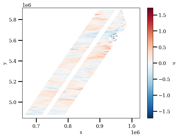
ds.u.plot()
[3]:
<matplotlib.collections.QuadMesh at 0x7e4fe61cb770>
Compute third order Isotropic Longitudinal SF
[ ]:
# Common parameters for structure function calculations
bin_r = np.logspace(np.log10(2000.), np.log10(1.0e6), 11)
bins = {'r': bin_r}

sf_kwargs = {
    "ds": ds,
    "bins": bins,
    "bootsize": {'y': 265, 'x': 69},
    "initial_nbootstrap": 60,
    "max_nbootstrap": 420,
    "step_nbootstrap": 40,
    "window_size_r": 8,
    "window_size_theta": 10,
    "backend": 'loky',
    "seed": 42
}
[4]:
%%time

iso_sf_lon = psf.get_isotropic_sf_2d(
    variables_names=["u", "v"],
    order=3,
    fun='longitudinal',
    convergence_eps=0.1,
    **sf_kwargs
)
Dimensions ('y', 'x') are already in the expected order
Dimension x has bootsize equal to or larger than dimension size. No bootstrapping will be done across this dimension.
Using bootsize: {'y': 265, 'x': 69}
Bootstrappable dimensions: ['y']
Single bootstrappable dimension (y). Using spacings: [1, 2]

============================================================
STARTING ISOTROPIC_SF WITH FUNCTION TYPE: longitudinal
Variables: ['u', 'v'], Order: 3
Confidence level: 0.95
============================================================


INITIAL BOOTSTRAP PHASE
Processing spacing 1 with 30 bootstraps
Processing spacing 2 with 30 bootstraps

CALCULATING BIN DENSITIES
Total points collected: 2586289999
Bins with points: 10/10
Marked 10 bins as converged (converged_eps)

STARTING ADAPTIVE CONVERGENCE LOOP
All bins have converged or reached max bootstraps!

FINAL CONVERGENCE STATISTICS:
  Total bins with data (>10 points): 10
  Converged bins: 10
  Unconverged bins: 0
  Bins at max bootstraps: 0

Creating output dataset...
ISOTROPIC SF COMPLETED SUCCESSFULLY!
============================================================
CPU times: user 1.58 s, sys: 126 ms, total: 1.7 s
Wall time: 50.5 s
Plot third order Isotropic Longitudinal SF
[5]:
# Create separate figures for better spacing and clarity
plt.figure(figsize=(10, 6))
# Structure Function with Confidence Interval
plt.plot(iso_sf_lon.r, iso_sf_lon.sf, 'b-', linewidth=2.5, label='Longitudinal Structure Function'+' '+'$\delta u_{LLL}$')

plt.fill_between(iso_sf_lon.r,
                iso_sf_lon.ci_lower,
                iso_sf_lon.ci_upper,
                alpha=0.3, color='blue')


# Formatting
plt.xlabel(r'$r$ [m]', fontsize=12, fontweight='bold')
plt.ylabel(r'$[m^{3}~s^{-3}]$', fontsize=12, fontweight='bold')
plt.title('Isotropic Longitudinal Structure Function with Confidence Intervals',
         fontsize=14, fontweight='bold', pad=10)
plt.legend(fontsize=11, frameon=True, facecolor='white', framealpha=0.9)
plt.grid(True, which='both', linestyle='--', alpha=0.6)
plt.xscale('log')

# Customize spines
ax = plt.gca()
for spine in ax.spines.values():
    spine.set_linewidth(1.5)

# Customize tick parameters
ax.tick_params(which='both', direction='in', width=1.2, length=5,
              labelsize=10, top=True, right=True)
ax.xaxis.set_major_formatter(ticker.LogFormatterSciNotation())

plt.tight_layout()

# --------------------------------------------------
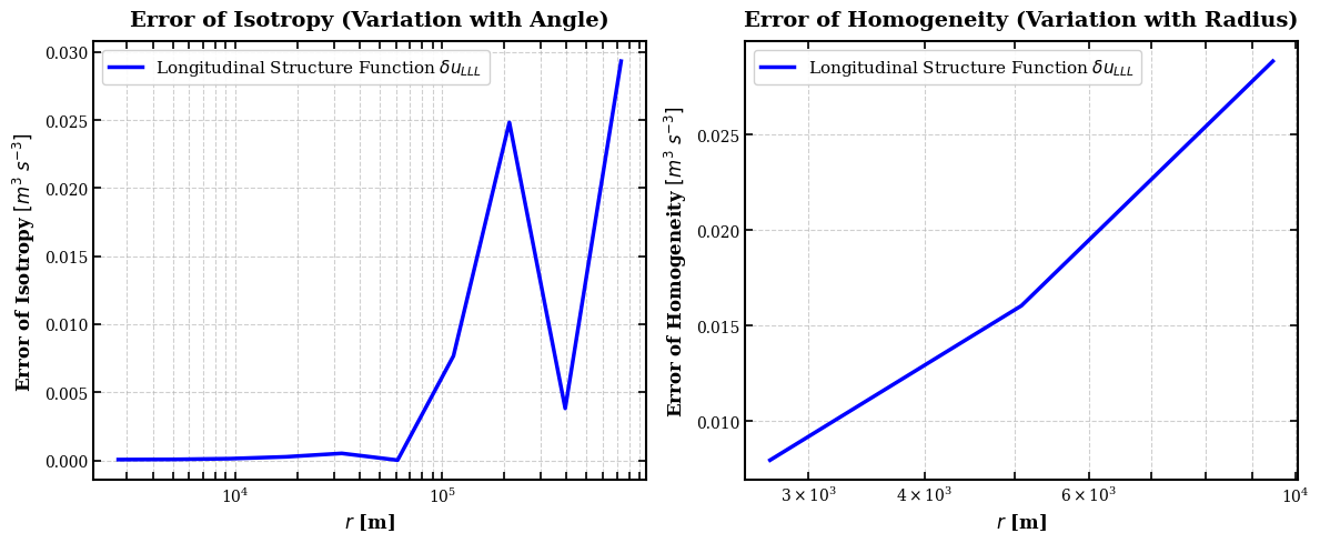
# Errors of Isotropy and Homogeneity
# --------------------------------------------------
plt.figure(figsize=(12, 5))

# Error of isotropy
plt.subplot(121)
plt.plot(iso_sf_lon.r, iso_sf_lon.error_isotropy, 'b-', linewidth=2.5,label='Longitudinal Structure Function'+' '+'$\delta u_{LLL}$')

plt.xlabel(r'$r$ [m]', fontsize=12, fontweight='bold')
plt.ylabel('Error of Isotropy'+' '+r'$[m^{3}~s^{-3}]$', fontsize=12, fontweight='bold')
plt.title('Error of Isotropy (Variation with Angle)',
         fontsize=14, fontweight='bold', pad=10)
plt.grid(True, which='both', linestyle='--', alpha=0.6)
plt.xscale('log')
plt.legend(fontsize=11, frameon=True, facecolor='white', framealpha=0.9)

# Customize spines and ticks
ax = plt.gca()
for spine in ax.spines.values():
    spine.set_linewidth(1.5)
ax.tick_params(which='both', direction='in', width=1.2, length=5,
              labelsize=10, top=True, right=True)
ax.xaxis.set_major_formatter(ticker.LogFormatterSciNotation())

# Error of homogeneity
plt.subplot(122)
plt.plot(iso_sf_lon.r_subset, iso_sf_lon.error_homogeneity, 'b-', linewidth=2.5,label='Longitudinal Structure Function'+' '+'$\delta u_{LLL}$')
plt.xlabel(r'$r$ [m]', fontsize=12, fontweight='bold')
plt.ylabel('Error of Homogeneity'+' '+r'$[m^{3}~s^{-3}]$', fontsize=12, fontweight='bold')
plt.title('Error of Homogeneity (Variation with Radius)',
         fontsize=14, fontweight='bold', pad=10)
plt.grid(True, which='both', linestyle='--', alpha=0.6)
plt.xscale('log')
plt.legend(fontsize=11, frameon=True, facecolor='white', framealpha=0.9)

# Customize spines and ticks
ax = plt.gca()
for spine in ax.spines.values():
    spine.set_linewidth(1.5)
ax.tick_params(which='both', direction='in', width=1.2, length=5,
              labelsize=10, top=True, right=True)
ax.xaxis.set_major_formatter(ticker.LogFormatterSciNotation())

plt.tight_layout()

plt.show()
Physical Interpretation: Third-Order Longitudinal Structure Function
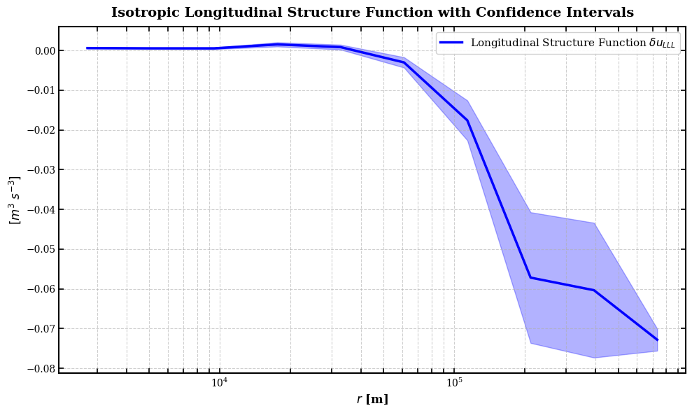
The third-order longitudinal structure function \(S_{LLL}(r) = \langle [\delta u_L]^3 \rangle\) is a key diagnostic for energy cascades in geostrophic turbulence. Key observations:
Negative values indicate an inverse energy cascade — energy flows from smaller to larger scales, which is characteristic of quasi-2D geostrophic turbulence in the ocean.
Positive values (if present at small scales) would indicate a forward cascade toward dissipation.
The magnitude relates directly to the energy flux rate \(\epsilon\) through the relation \(S_{LLL} = -\frac{3}{2} \epsilon r\) in the inertial range.
The confidence intervals (shaded region) quantify statistical uncertainty, which increases at the largest scales due to fewer independent samples.
Compute advective SF
[6]:
%%time

iso_sf_adv = psf.get_isotropic_sf_2d(
    variables_names=["u", "v", "adv_u", "adv_v"],
    order=1,
    fun='advective',
    convergence_eps=1.0e-7,
    **sf_kwargs
)
Dimensions ('y', 'x') are already in the expected order
Dimension x has bootsize equal to or larger than dimension size. No bootstrapping will be done across this dimension.
Using bootsize: {'y': 265, 'x': 69}
Bootstrappable dimensions: ['y']
Single bootstrappable dimension (y). Using spacings: [1, 2]

============================================================
STARTING ISOTROPIC_SF WITH FUNCTION TYPE: advective
Variables: ['u', 'v', 'adv_u', 'adv_v'], Order: 1
Confidence level: 0.95
============================================================


INITIAL BOOTSTRAP PHASE
Processing spacing 1 with 30 bootstraps
Processing spacing 2 with 30 bootstraps

CALCULATING BIN DENSITIES
Total points collected: 2103478976
Bins with points: 10/10
Marked 10 bins as converged (converged_eps)

STARTING ADAPTIVE CONVERGENCE LOOP
All bins have converged or reached max bootstraps!

FINAL CONVERGENCE STATISTICS:
  Total bins with data (>10 points): 10
  Converged bins: 10
  Unconverged bins: 0
  Bins at max bootstraps: 0

Creating output dataset...
ISOTROPIC SF COMPLETED SUCCESSFULLY!
============================================================
CPU times: user 1.45 s, sys: 121 ms, total: 1.57 s
Wall time: 39.4 s
Plot Advective SF
[7]:
# Create separate figures for better spacing and clarity
plt.figure(figsize=(10, 6))
# Structure Function with Confidence Interval
plt.plot(iso_sf_adv.r, iso_sf_adv.sf, 'b-', linewidth=2.5)

plt.fill_between(iso_sf_adv.r,
                iso_sf_adv.ci_lower,
                iso_sf_adv.ci_upper,
                alpha=0.3, color='blue')


# Formatting
plt.xlabel(r'$r$ [m]', fontsize=12, fontweight='bold')
plt.ylabel(r'$\delta u.\delta ADV~[m^{2}~s^{-3}]$', fontsize=12, fontweight='bold')
plt.title('Isotropic Advective Structure Function with Confidence Intervals',
         fontsize=14, fontweight='bold', pad=10)
plt.grid(True, which='both', linestyle='--', alpha=0.6)
plt.xscale('log')

# Customize spines
ax = plt.gca()
for spine in ax.spines.values():
    spine.set_linewidth(1.5)

# Customize tick parameters
ax.tick_params(which='both', direction='in', width=1.2, length=5,
              labelsize=10, top=True, right=True)
ax.xaxis.set_major_formatter(ticker.LogFormatterSciNotation())

plt.tight_layout()

# --------------------------------------------------
# Errors of Isotropy and Homogeneity
# --------------------------------------------------
plt.figure(figsize=(12, 5))

# Error of isotropy
plt.subplot(121)
plt.plot(iso_sf_adv.r, iso_sf_adv.error_isotropy, 'b-', linewidth=2.5)

plt.xlabel(r'$r$ [m]', fontsize=12, fontweight='bold')
plt.ylabel('Error of Isotropy'+' '+r'$[m^{2}~s^{-3}]$', fontsize=12, fontweight='bold')
plt.title('Error of Isotropy (Variation with Angle)',
         fontsize=14, fontweight='bold', pad=10)
plt.grid(True, which='both', linestyle='--', alpha=0.6)
plt.xscale('log')

# Customize spines and ticks
ax = plt.gca()
for spine in ax.spines.values():
    spine.set_linewidth(1.5)
ax.tick_params(which='both', direction='in', width=1.2, length=5,
              labelsize=10, top=True, right=True)
ax.xaxis.set_major_formatter(ticker.LogFormatterSciNotation())

# Error of homogeneity
plt.subplot(122)
plt.plot(iso_sf_adv.r_subset, iso_sf_adv.error_homogeneity, 'b-', linewidth=2.5)
plt.xlabel(r'$r$ [m]', fontsize=12, fontweight='bold')
plt.ylabel('Error of Homogeneity'+' '+r'$[m^{2}~s^{-3}]$', fontsize=12, fontweight='bold')
plt.title('Error of Homogeneity (Variation with Radius)',
         fontsize=14, fontweight='bold', pad=10)
plt.grid(True, which='both', linestyle='--', alpha=0.6)
plt.xscale('log')

# Customize spines and ticks
ax = plt.gca()
for spine in ax.spines.values():
    spine.set_linewidth(1.5)
ax.tick_params(which='both', direction='in', width=1.2, length=5,
              labelsize=10, top=True, right=True)
ax.xaxis.set_major_formatter(ticker.LogFormatterSciNotation())

plt.tight_layout()

plt.show()
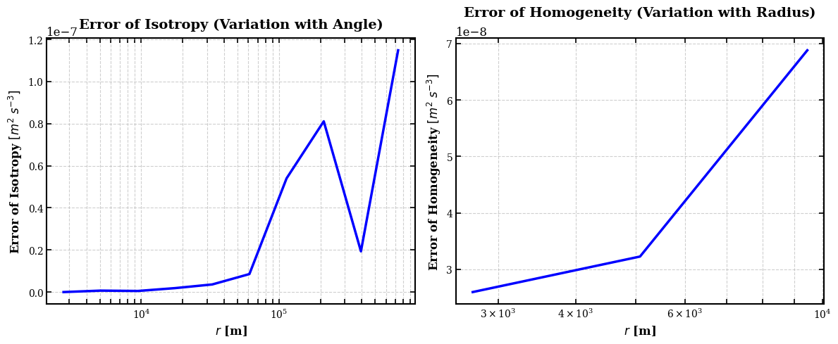
Physical Interpretation: Advective Structure Function
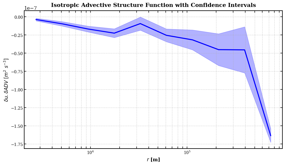
The advective structure function \(\langle \delta \mathbf{u} \cdot \delta \mathbf{A} \rangle\) provides an alternative measure of the energy cascade that is particularly useful for anisotropic flows:
Unlike \(S_{LLL}\), the advective SF does not assume isotropy and can capture energy transfer even when the flow has preferred directions.
Negative values again indicate an inverse cascade (energy moving to larger scales).
The advective SF is related to energy flux by \(\epsilon = -\frac{1}{2} \langle \delta \mathbf{u} \cdot \delta \mathbf{A} \rangle\).
Comparing the two methods (longitudinal vs advective) provides a consistency check and reveals potential anisotropies in the cascade.
Estimate Cascade rates
In 2D quasi-geostrophy, the third order longitudinal structure function \(\delta u_{LLL}\) and the advective structure function \(\delta u . \delta ADV\) are related to inverse cascade rates:
\(\rm \epsilon = -2\delta u_{LLL}/3r\)
\(\rm \epsilon = -\delta u.\delta ADV/2\)
[8]:
eps_lon = -2*iso_sf_lon.sf/(3*iso_sf_lon.r)
eps_adv = -iso_sf_adv.sf/2.0
Plot Cascade rates
[9]:
# Create separate figures for better spacing and clarity
plt.figure(figsize=(10, 6))
# Structure Function with Confidence Interval
plt.plot(iso_sf_adv.r, eps_lon, 'b-', linewidth=2.5,label=r'$\delta u_{LLL}$')
plt.plot(iso_sf_adv.r, eps_adv, 'r-', linewidth=2.5,label=r'$\delta u.\delta ADV$')


# Formatting
plt.xlabel(r'$r$ [m]', fontsize=12, fontweight='bold')
plt.ylabel(r"Inverse energy cascade rate [m$^2$s$^{-3}$]", fontsize=12, fontweight='bold')
plt.legend()
plt.grid(True, which='both', linestyle='--', alpha=0.6)
plt.xscale('log')
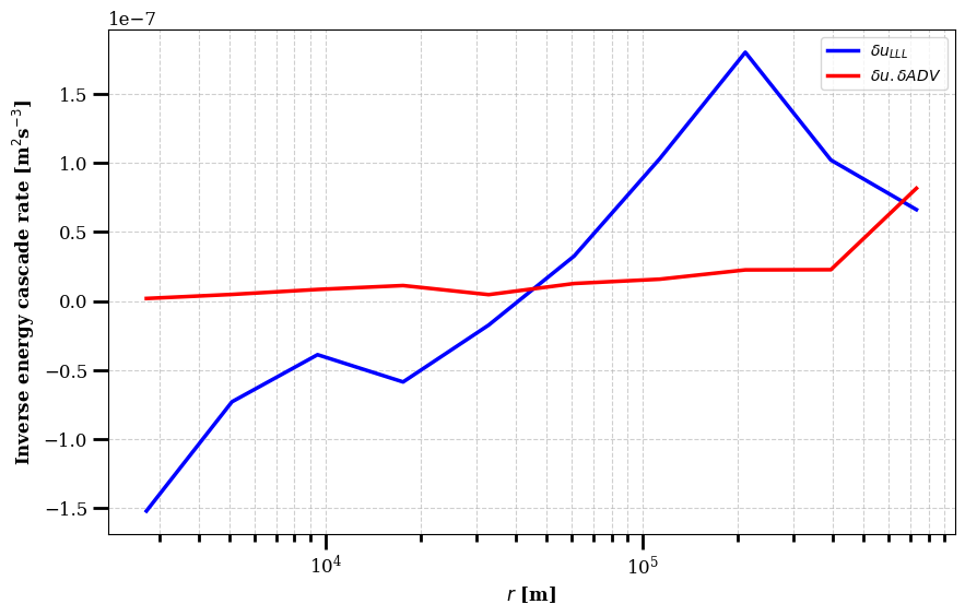
Physical Interpretation: Energy Cascade Rates
This figure compares the energy cascade rates derived from both structure function methods:
Agreement between methods validates the robustness of the cascade rate estimate and suggests the flow is approximately isotropic.
Constant \(\epsilon\) with scale in the inertial range indicates a self-similar cascade following Kolmogorov-like dynamics.
The sign of \(\epsilon\) confirms the direction of energy transfer: negative for inverse cascade (toward larger scales), positive for forward cascade (toward dissipation).
Typical values of \(O(10^{-10})\) to \(O(10^{-9})\) W/kg are consistent with mesoscale eddy energetics in the ocean.
This analysis demonstrates how SWOT altimetry data can quantify the ocean’s kinetic energy budget at mesoscale and submesoscale ranges.
[ ]: